
(Re)Tallying the Tightening
(Re)Tallying the Tightening
We refine our estimates of March's impact.

Summary
We do a more granular analysis of the impact of March’s banking stress, and revise downwards the total hit to growth and inflation we expect to result. First, we develop a proxy for concerns around the banking sector. We then use this proxy to evaluate the impact of banking concerns on different types of lending, and on lending overall. We anticipate Commercial & Industrial lending growth to decelerate notably, and see a more persistent but less severe drag on real estate and consumer lending growth. We feed our more objective lending growth assumptions into our macro model from “Tallying the Tightening” – the results suggest a more modest macro impact than we initially anticipated.
Roadshow: 24th - 28th April
Our Q2 roadshow will run during this week, and we’re offering clients and prospects:
- 30 minute outlook presentations with Q&A for institutions.
- A webinar consisting of a 30 minute presentation, with an additional 15 mins for Q&A, on Thursday 27th at 3pm London time / 4pm CEST / 10am New York.
To register your interest please reach out on here or to mailto:robert.brown@ashridgemacro.com?subject=Roadshow, specifying whether you’re interested in joining the webinar or receiving an institutional presentation.
A New Proxy for Banking Sector Concern
In “Tallying the Tightening” we provided a rough ballpark estimate of the macro impact of March’s banking sector panic, under the assumption that tighter lending conditions would likely result from March’s bout of concern. We examined several scenarios to come up with our somewhat subjective baseline. To refine our estimates and improve upon our prior work, we constructed a proxy for generalized concern around the health of the banking sector.
To construct our proxy, we calculated the daily performance of a basket of individual bank equities versus the broader market. We took data on a large and diverse set of US banks, including GSIBS/large banks, regional banks and listed community banks. We then took an un-weighted cross-sectional average of the relative performance and estimated the stochastic volatility of that average. We took this measure as our proxy for concerns around the health of the banking sector, such as those seen in March.

Our proxy exhibits encouraging co-movement with proxies for broader financial stress, particularly during periods of heightened stress/concern. The plots below plot our indicator versus the St Louis Fed’s Financial Stress Index, the TED Spread and the VIX, with the latter two logged for easier visualization. Local regression lines are overlaid. Our indicator co-moves positively with all three variables.
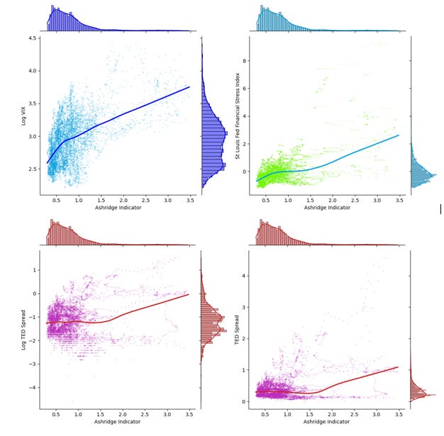
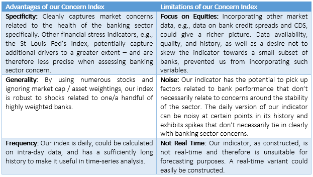
The intention of our metric is to capture generalized concerns about the health/stability of the banking sector, which may have a macro impact over time if they result in more risk-averse asset-liability management on the part of banks. Conceptually, the scope of our metric is slightly different from financial stress indices, and market variables like TED and Libor-OIS spreads. Our approach has advantages and drawbacks.
Our indicator captures March concerns well, increasing in the run-up to and aftermath of SVB’s failure and peaking on 13th March. The indicator reached a local trough around the turn of the year and had already risen somewhat through January and February. During March, the concern indicator spiked by around one point. It has since retraced around 2/3 of that spike, consistent with the view that banking sector concerns are off their peak.
Lending Behaviour After Bouts of Concern
For the next stage in our analysis, we used our proxy to examine how bank lending behaviour evolves following episodes of banking sector concern. Our hypothesis was that, even absent further material failures, elevated concern about bank solvency / viability should lead to more conservative lending, as banks seek to manage balance sheets with a greater degree of risk aversion and caution. As in Tallying the Tightening, we employ a Bayesian VAR with time varying parameters and stochastic volatility, estimating a series of distinct models for different components of bank lending.
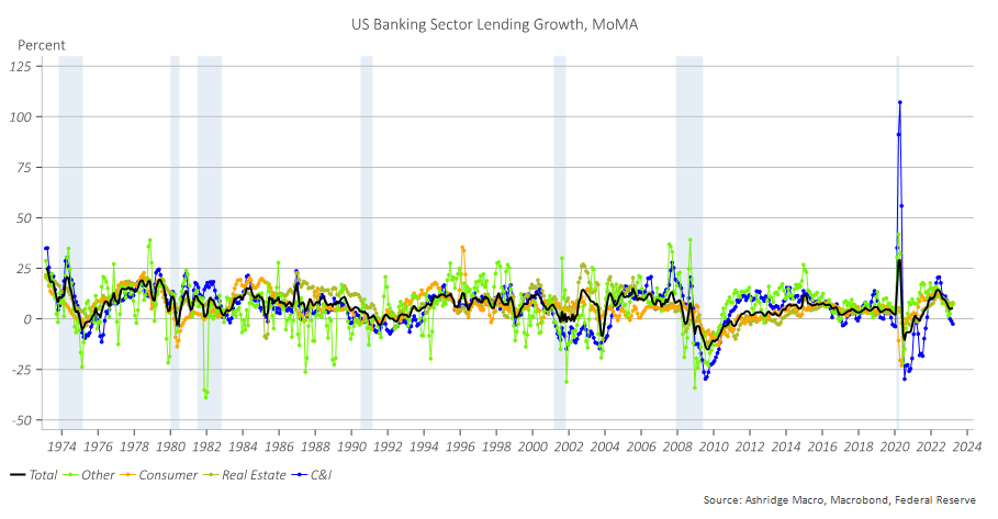
We model break-adjusted and seasonally adjusted month-over-month annualized growth rates for total bank lending and four subdivisions of bank lending (total real estate lending, CRE, commercial & industrial, consumer and “all other loans and leases[1]” – hereafter “other”), sourced from the H8 release[2]. Our data is monthly – we incorporate the monthly average of our concern proxy.
We included a monthly growth proxy (the Chicago Fed national activity index), the Federal Funds rate and the slope of the yield curve as controls. We use the first five years’ worth of data as a training sample to calibrate our priors – data which is then discarded[3].
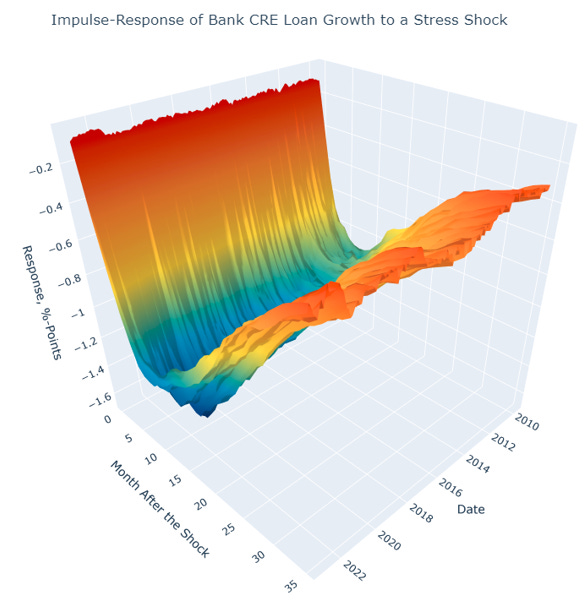
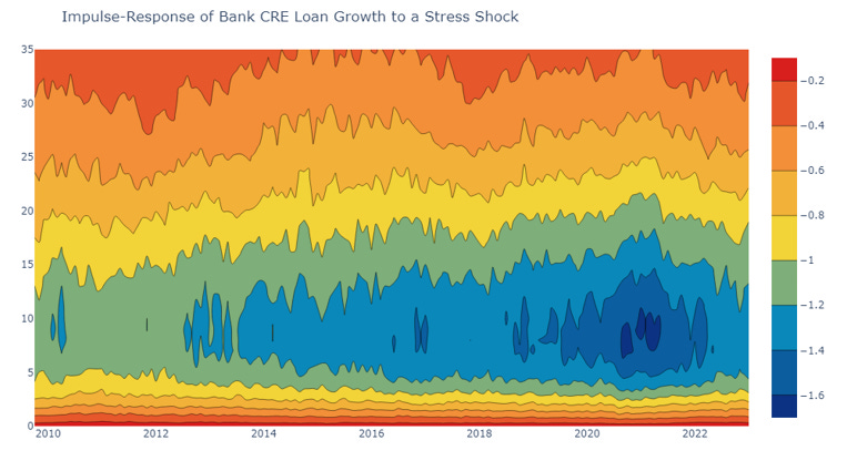
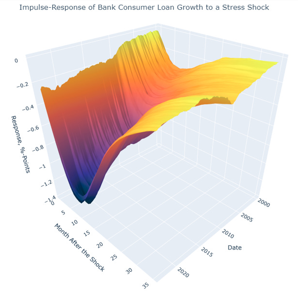
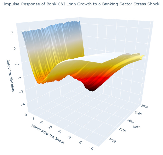
The charts below plot the deceleration in lending growth, in %-points annualized, after a unit positive shock to our banking concern proxy. A priori, we would anticipate a negative impulse response function. The x-axis shows the number of months after the stress shock and the y-axis captures the variation in the response through time. A secondary contour plot is also presented.
Overall Lending
Somewhat counterintuitively, the impulse-response of lending growth suggests a statistically insignificant acceleration immediately after the shock.
After the initial insignificant rise, the IRF begins to display the expected negative sign and the deceleration in lending growth resulting from the concern shock becomes statistically significant. The deceleration builds over time.
The deceleration is at its greatest extent around eight months after the stress shock, by which time the annualized rate of lending growth will have slowed by around 80bps. The pace of lending growth then gradually normalizes.
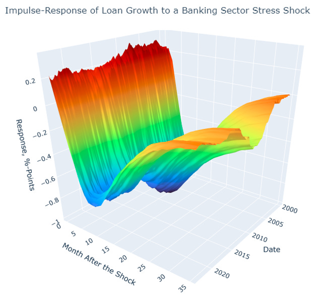
The impact of concern shocks on overall lending has moderated over time. During the global financial crisis, bank concern shocks produced a sharper deceleration than currently, and also exerted a more persistent drag on lending growth.

Real Estate Lending
Shocks begin to exert downward pressure on real estate lending growth fairly rapidly, per our estimated impulse-responses. The trough in growth occurs 5-6 months after the shock.
A degree of time-variation is in evidence, with shocks exerting a greater degree of downward pressure towards the end of the sample, as well as around the time of the global financial crisis.
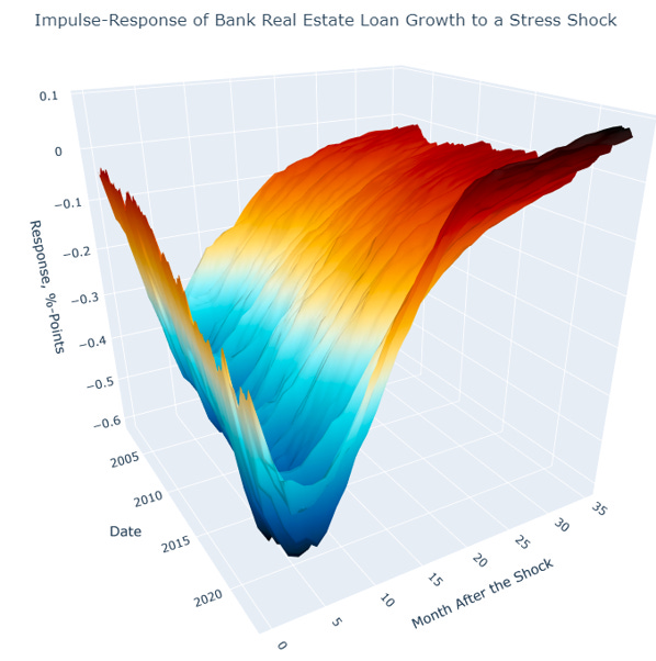

Commercial real estate lending slows less rapidly after a concern shock than overall real estate lending - the peak downward effect occurs after 7-8 months.
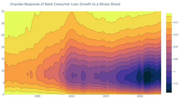
Consumer Lending
Consumer lending declines less rapidly than some other components after a banking sector concern shock, with the trough occurring 6-7 months after the shock.
There is notable time-variance in the impulse response – after the financial crisis, a banking sector concern shock of the same magnitude produced a deeper and more persistent deceleration in consumer lending growth.
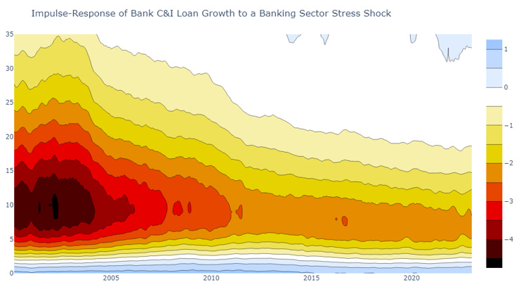
Commercial & Industrial Lending
Initially, Commercial & industrial lending accelerates after a shock – but this acceleration is not statistically significant.
A statistically significant decline occurs subsequently, with the peak effect coming through after about 6 months.
As with other types of lending there is some evidence of time-variation in the impulse response, albeit in the opposite direction – the impact on C&I lending growth appears less severe post-GFC versus before.
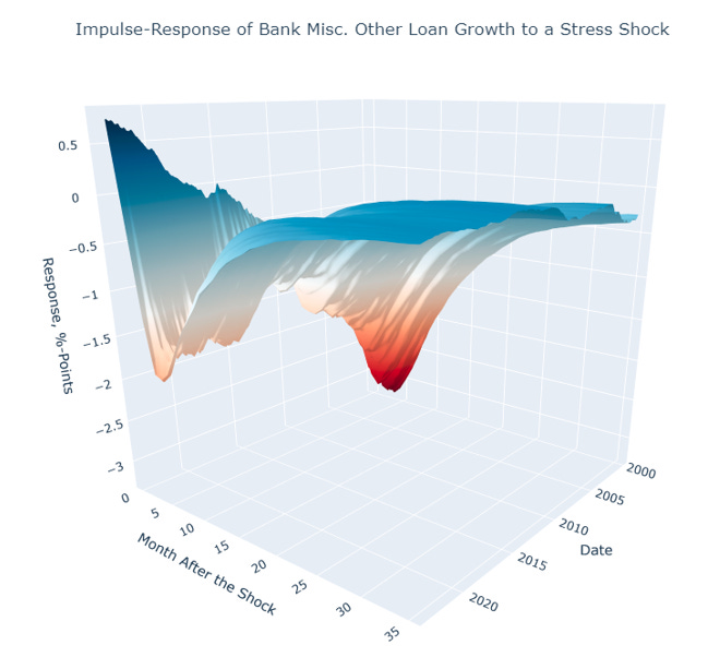
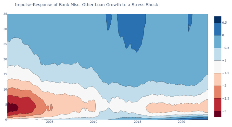
All Other Loans & Leases
The response of growth in all other loans and leases displays an insignificant initial acceleration before a statistically significant deceleration.
The peak impact comes after around four months.
This impulse-response displays quite a bit of time variance. Much greater peak effects were seen pre-GFC, these then damped down during the early 2010s, before increasing again.
As a robustness check, we re-estimated each model multiple times employing different prior and ordering assumptions as well as using alternative proxies for banking sector stress. Alternative proxies generally produced impulse response functions which were less consistent with macro theory overall. Alternative priors and ordering did not change our conclusions materially.
Plugging in the March Shock
We next use our IRF analysis to estimate the total impact of March’s banking sector concerns on bank lending growth. To do this, we take the most modern impulse response estimates, and feed through the total moves in our banking sector stress proxy over the course of March and April. By incorporating April data, we capture the moderation of banking sector concerns from their highs in March.
The first plot below shows the deceleration in lending growth implied by the concern shocks. Recent concerns should weigh on all categories of lending over the coming months. With the exception of the catch-all “all other loans and leases” category, commercial and industrial lending growth should be dampened most heavily. The impact on real estate lending should be smaller and less persistent, and the impact on consumer lending growth shallower than some other categories, but more drawn out.

The larger response in C&I and “all other” lending tallies with historical data on the relative volatilities of each category of lending. The historical standard deviation of “all other” growth is around 2.2x that of total lending – C&I lending growth is around 1.6x, and residential and consumer lending both have standard deviations about 0.9x that of the total.
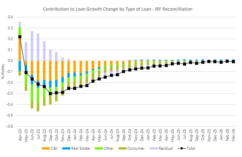
By using the shares of each lending category in banks’ total lending, we can back out contributions to the total lending growth deceleration from each lending category. By September 2023, the peak of the direct impact of the concern shock should be in – at which point we estimate the MoMA growth rate of overall lending will be around 30bps lower than absent the Q1 banking sector concerns.
Of this 30bps reduction:
18bps will be driven by slowing C&I lending.
Around 8bps will be driven by slower consumer lending and slowing growth rates in other types of lending.
The impact on real estate lending will be past its peak – 6bps of the deceleration in total lending growth will be driven by real estate lending.
Our decomposition includes a discrepancy – relatively large at short horizons but smaller further out – reflecting the fact that our IRF for total lending does not tally exactly with the weighted sum of its “parts”. This reflects imperfections in our modelling strategy, as well as potentially capturing some fundamental behavioural factors such as endogenous changes in bank lending preferences after a shock.
Updating Our Base Case for the GDP and Inflation Impact
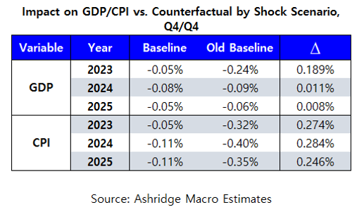
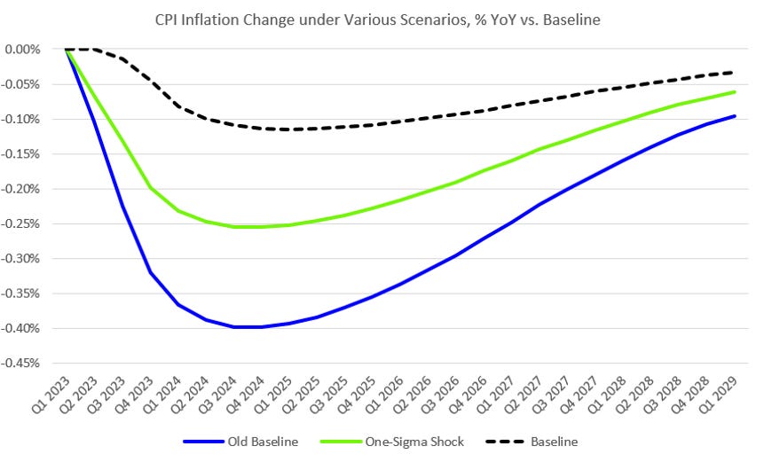
In Tallying the Tightening, we estimated, as a ballpark, that the effects of the March concerns could reduce GDP growth this year by around 25bps, and inflation by around 36bps. To derive a higher-conviction and less subjective estimate, we map our projected impact on bank lending into a total, economy-wide lending impact[4], and then plug the results into the model for GDP and inflation estimated in Tallying the Tightening.
Our more detailed analysis revises our baseline substantially upwards – the impact of March volatility on inflation and GDP now appears smaller than initially thought. Of course, this follow-up work also benefits from more information than our previous effort, in particular capturing the damping down of concerns from their peak in the latter part of March and through April thus far.

[1] Fed defines as: “Includes loans for purchasing or carrying securities, loans to finance agricultural production, loans to foreign governments and foreign banks, obligations of states and political subdivisions, loans to nonbank depository institutions, loans to non-depository financial institutions, unplanned overdrafts, loans not elsewhere classified, and lease financing receivables.”
[2] It is critical to break-adjust the H8 data, leading to our preference for modelling growth rates over levels. This is because definitional changes and other methodological/technical factors have driven large jumps/dips in the data which would otherwise skew results. As an example, Ghazaly and Gopalan (2010) discuss how methodological changes caused a dramatic jump in unadjusted bank consumer loan numbers in 2010.
[3] We expanded our training sample slightly for the real estate model, in order to set a slightly tighter prior. Initial variants of the model with a 5-year training sample displayed strange behaviour, which addition of further controls could not remove.
[4] We use an auxiliary regression model to map our bank lending shock into a total, economy-wide lending shock. Our definition of “total lending” includes essentially all bank and non-bank lenders to the US economy – incorporating things like credit unions and peer-to-peer lending which banking sector lending alone wouldn’t capture, but which are nevertheless relevant for growth and inflation. The auxiliary regression estimates the elasticity of total lending to bank lending – in general, total lending exhibits less volatility than bank lending.